Computing Global Sensitivity Measures from Given Samples
Elmar Plischke
Institute of Disposal Research
Clausthal University of Technology
This is handcrafted (X)HTML+MathML. You have been warned if your browser chokes on it.
If you're using IE+MathType, you might want to look at
this page with xht suffix
instead.
Global Sensitivity Measures
We are investigating computationally effective methods for Sensitivity Analysis.
(Saltelli et al., 2006) defines this as
"Sensitivity analysis is the study of how the variation on the output of a model (numerical or otherwise)
can be apportioned, qualitatively or quantitatively,
to different sources of variation, and of how the given model depends upon the information fed into it."
Methods for the Sensitivity Analysis of Model Outputs
- Types of input uncertainty must be known
- Designed samples can be used to exploit the parameter space optimally:
factorial designs, Latin hypercube samples, quasi Monte-Carlo samples
- Simulation model must be available
- If computing time permits, precision to the last digital place is achievable
This is the current favourable choice for computing an importance measure.
This approach may be computationally expensive as there are model-evaluations in the loop!
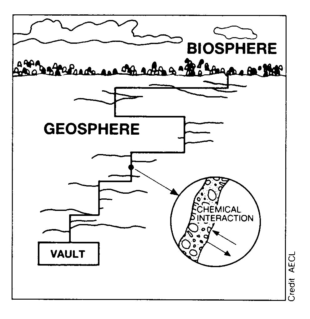
Sensitivity Analysis in Disposal Research
In Disposal Research, there is the concept of a
Safety Case which might be described as a systematic
collection of arguments demonstrating the safety of a repository for hazardous or
radioactive waste in the deep underground.
For this demonstration, model calculations predicting the risk are needed. But
- parameter and data are uncertain: limited knowledge about properties of host rock, excavation damage
- the model is uncertain: limited process understanding (microbes,
thermo-hydraulic-mechanic coupling, sorption processes)
- the scenario is uncertain: Further evolution of a repository site is not exactly predictable
(ice ages, behaviour of barriers and materials in large timescales)
We need a sensitivity analysis to support the safety case to
show the robustness of our proposed strategy against uncertainties.
General approach
A deterministic model of nuclide transport is embedded into a probabilistic framework to
study the variability in the inputs and outputs.
| Deterministic model | Probabilistic framework |
 |
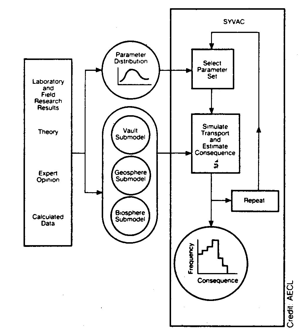 |
This approach can be found in many applied disciplines where simulation models are used and
their outcomes have to be judged which forms part of a larger decision process.
Condensing Scatterplots into Numbers
Given the input sources and the outputs (model runs or measurements)
we consider the problem of measuring the "degree of information" available in a scatterplot
of the data for one input parameter (or more) plotted against the output data.
As a goal, we want to use one and the same sample for computing
- linear,
- functional, and
- density-based
sensitivity measures. This sample may already be available from an
uncertainty analysis, requiring only minimal assumptions about the sample
design. This breaks with the tradition of a sensitivity analysis with
a simulation model in the loop.
A sensitivity analysis is a reduction of a functional or statistical dependency to
a number: It is always a question which kind of information is lost during this analysis step.
In most cases, our visual intuition is able to judge this question.
Example: The Ishigami test function
This test function is widely used in sensitivity analysis. It is given by
where the parameters
are independently uniformly distributed. We use it with a fourth factor which is a dummy.
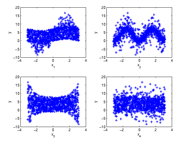
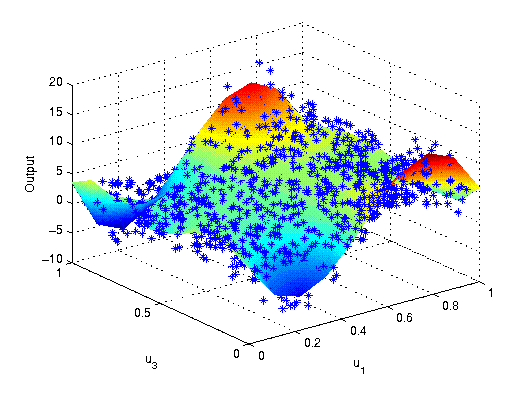
Scatterplots for the Ishigami function (including a dummy parameter)
In the following we will attribute different sensitivity indicators to these scatterplots.
Linear Regression
A widely used measure of association is given by
Pearson's product-moment correlation coefficient
where
|
| pairs of data |
| | mean of s |
| | mean of s |
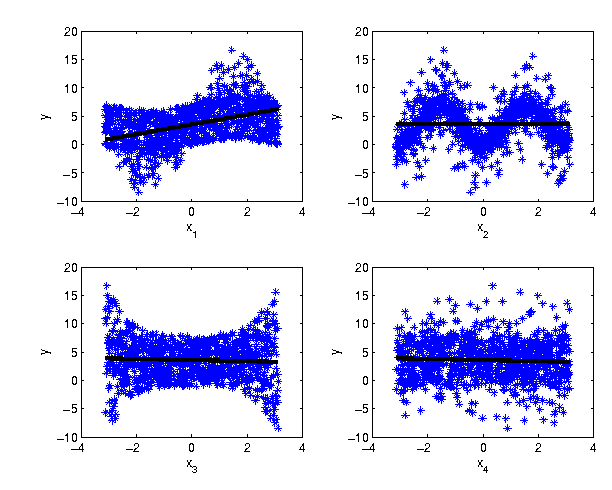 The correlation coefficient is the product of the linear regression coefficients (gradients)
and
In the example, the linear trend is only a suitable measure for the first
factor. Factor 2 and 3 show nonrandom influences on the output that
are not captured by the zero indicator value.
The correlation coefficient is the product of the linear regression coefficients (gradients)
and
In the example, the linear trend is only a suitable measure for the first
factor. Factor 2 and 3 show nonrandom influences on the output that
are not captured by the zero indicator value.
| Parameter | 1 | 2 | 3 | 4 |
| |
0.1936 | 0.0000 | 0.0026 | 0.0026 |
Linear regression is often used in sensitivity analysis.
However, as (Pearson, 1912) notes
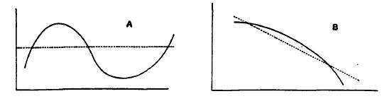 "Nothing can be learnt of association by
assuming linearity in a case with a regression line (plane, etc.) like A,
much in a case like B."
"Nothing can be learnt of association by
assuming linearity in a case with a regression line (plane, etc.) like A,
much in a case like B."
Measures of dependency stronger than linear correlation
We can strengthen this approach to derive sensitivity indicators
by using
- Logarithmic transformations, rank regressions
- General linear models
- Variance-based sensitivity measures
- Density-based sensitivity methods
We discuss variance and density sensitivity methods.
Correlation Ratios
Knowing of the deficiencies of linear regression based indicators, (Pearson, 1905)
introduced the Correlation Ratio (CR).
Given data pairs of input and output values, the CR is obtained by the following steps.
- Classify the input data
using a suitable partition
- Compute the class means of the corresponding output data
- Compute the ratio of the variance between the classes and of the empirical
variance of
In particular, let use define
with .
Then the CR is given by
.
The Correlation Ratio is using a regression model which consists of step functions on a given class partition.
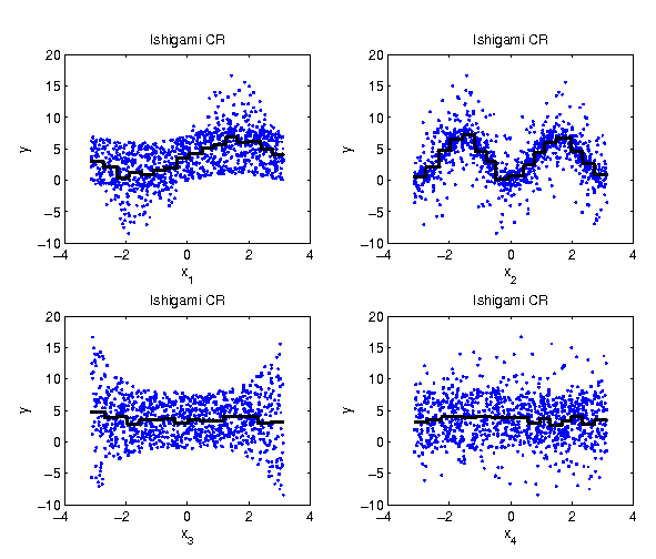
Plotting the class means
As a visual feedback, we plot the class means into the scatterplot. This is an
approximation of the non-parametric regression curve.
|
Parameter | 1 | 2 | 3 | 4 |
| |
0.3191 | 0.4138 | 0.0188 | 0.0148 |
First Order Effect
(Kolmogorov, 1933) identifies the Correlation Ratio as an estimate of
the quotient between the variance of the conditional expectation of
the output given the input and the unconditional variance of the output,
where is the input random variable and
is the output random variable.
This quantity is called first order effect,
main effect, or Sobol' index .
It is an example of a variance-based global sensitivity measure.
Estimators for the First Order Effect
If is an
estimate of
the regression curve
(local mean, "backbone" of the scatterplot)
then the first order effect can be estimated by
.
Hence this quantity measures the goodness-of-fit for the (non-linear)
model prediction
.
How to choose
?
For smoothing the scatterplots
we are free to choose a suitable regression model
from the toolbox for non-linear/non-parametric regression:
- Affine linear regression models
- Step functions (Pearson, 1905)
- (Piecewise) polynomials, splines
- Orthogonal basis of polynomials (Rabitz & Alis, 1999)
- Harmonic functions (Plischke, 2010)
- Wavelet decompositions
- Regression in orthogonal function spaces
- Moving averages (Doksum & Samarov, 1995)
- LOESS/LASSO/ACOSSO smoothing
- ...
Clearly, a linear regression model would yield
as an estimator of .
Example - Moving Averages
Let us try a moving window to compute a local mean for .
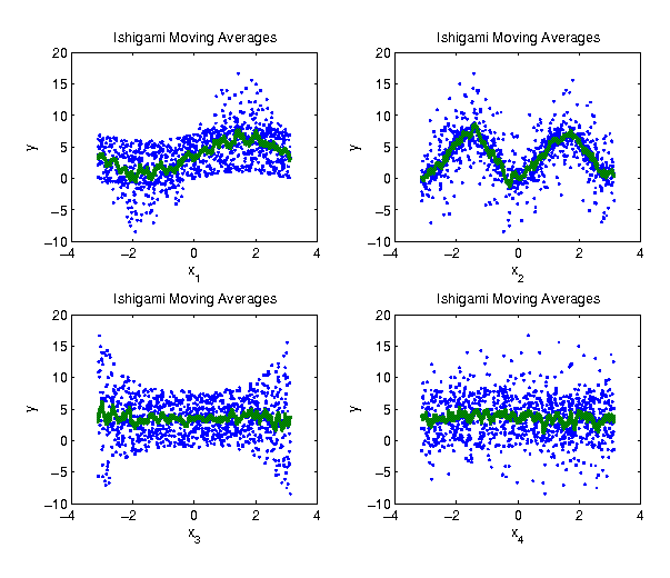
| Parameter | 1 | 2 | 3 | 4 |
| |
0.3499 | 0.4564 | 0.0616 | 0.0420 |
The window for the moving average is too small: the regression curve is jiggling.
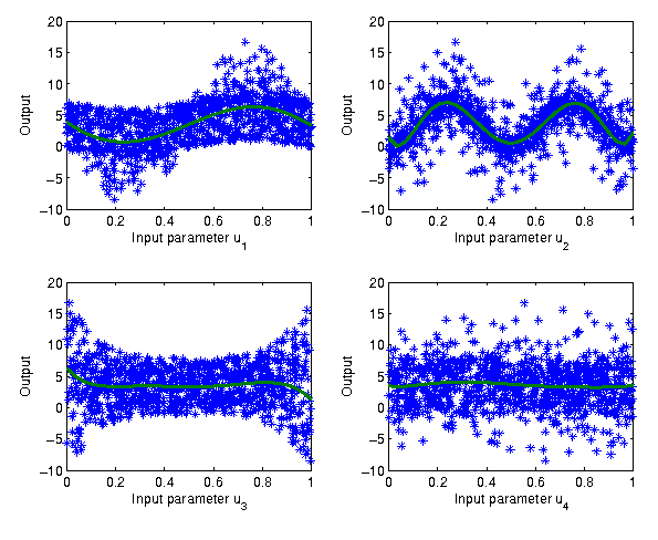
Example - Orthogonal Polynomials
Instead of fitting a linear dependency, we can fit a polynomial
model. If we use a orthogonal family of polynomials then the
computation of the conditional variances is simplified by Parseval's
theorem (which is a Pythagoras theorem for functions):
We just have to form the sum of squares of the computed/selected
coefficients.
|
Parameter | 1 | 2 | 3 | 4 |
| |
0.3107 | 0.4500 | 0.0280 | 0.0070 |
Orthogonal Polynomials: Higher order effects
This polynomial regression model can also contain interacting
terms. With their help, higher order sensitivity indices can be computed which are based on the following regression model.
The combination of and
contributes 0.2442 of output variance.
Fourier Amplitude Sensitivity Test (FAST)
The state of the art of
computing first order, higher order and/or total effects consists of using one of
- Ishigami/Saltelli/Homma
- Sobol'
- Jansen Winding Stairs
- Fourier Amplitude Sensitivity Test (FAST)
- Random Balance Design (RBD)
All these methods need special sampling schemes or repeated model evaluations.
(Cukier et al., 1973) introduced the FAST for Sensitivity Analysis.
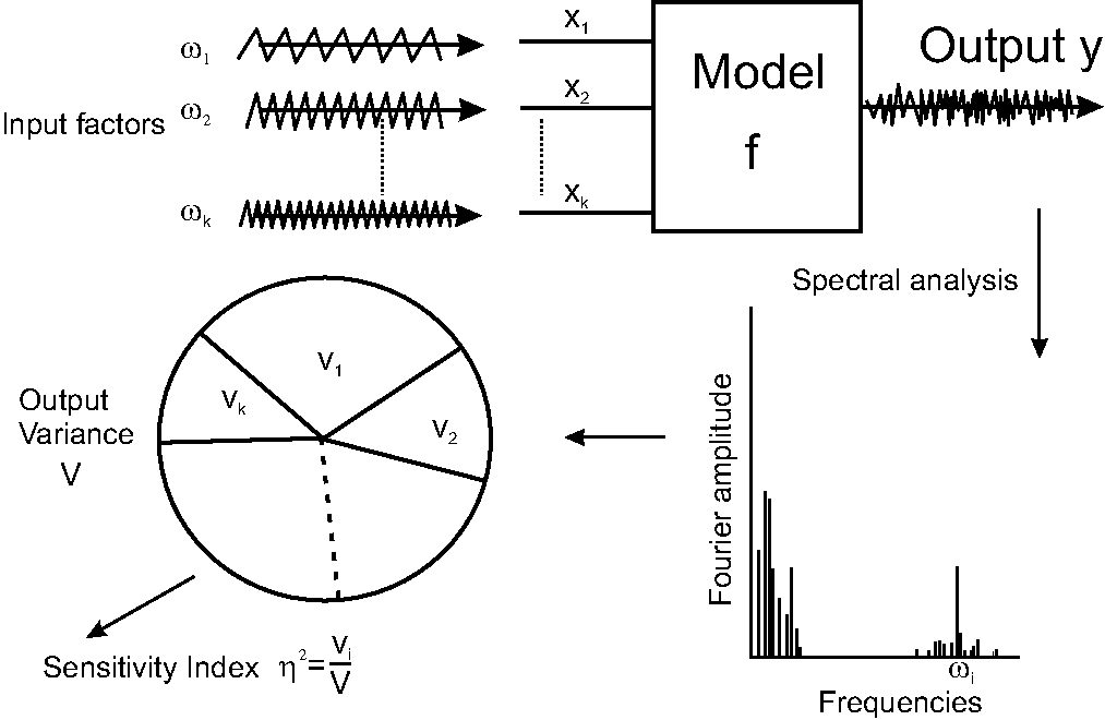
Each input factor is associated with a certain
frequency in the
specially design input sample. All resonances to this frequency in
the corresponding output sample are then attributed to the first order
effect of this factor.
FAST with sample size 8192
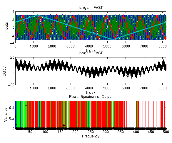
The Ishigami function analysed with FAST: Here factor 1 is associated with
frequency ,
factor 2 with ,
and factor 3 with . The
middle plot shows the output response and the lower plot its
frequency spectrum. Blue frequencies contribute to first order
effects, green to second order effects and red to third order
effects. For the first order effects of factor 1 we find two active
coefficients, the first one with approx. 20% being the only one
identified by linear regression. An additional coefficient of approx. 10%
would pass the linear regression unnoticed.
For the second factor,
the contributions are only visible in the fourth higher harmonic,
hence a linear regression predicts a zero influence. Factor 3
shows no first order effects, but second order effects with factor 1.
First and selected second order effects from FAST
|
Parameter | 1 | 2 | 3 | 4 | 1,3 |
|
0.3076 | 0.4428 | 0.0000 | 0.0000 | 0.2435 |
The sample constructed for FAST is not reusable.
As the sum is almost 100%, all of the output variance accounted for.
Some noteworthy points from FAST:
- Artificial timescale is coded by the position of the realisations in the sample
- The conditional expectations are computed via selection of resonating frequencies,
and higher harmonics
- Variance is given by the sum of squares of the frequencies due to Parseval's
Theorem for orthonormal transformation
- Effects caused by several parameters can be resolved by the
Supposition Principle which involves frequencies
and higher harmonics
Computationally efficient FAST-inspired Methods
How to combine the pro's from FAST into a computationally efficient method?
An example for such a FAST-inspired method could be based on the following decisions:
|
Artificial timescale |
Sort the output data using the input data of interest as key |
| Suitable orthogonal transformation | bisect the data using
Haar wavelet decomposition |
| Regression curve | First few coefficients of the transformed,
reordered output values |
We don't need a back-transformation because of orthonormality of the transformation.
The Haar wavelet decomposition transforms an adjacent data pair into midpoint and (signed) radius
and repeats this recursively for the midpoints.
MATLAB: Haar wavelets
With only a few lines of MatLab we can implement the program sketched above.
M = 5; 				% Higher harmonics
[xr,index] = sort(x); yr = y(index);
allcoeff = wavetrafo(yr);
Vi = sum(allcoeff(1+1:(2^M),:).^2);
V  = sum(allcoeff(2:end,:).^2);
etai = Vi./V;

function y=wavetrafo(x)
%WAVETRAFO Haar wavelet transformation.
[n,k]=size(x);
 if(n==1), y=x;  else
   sums = x(1:2:end,:)+x(2:2:end,:);
   diffs= x(1:2:end,:)-x(2:2:end,:);
   y=[ wavetrafo(sums); diffs]/sqrt(2);
 end
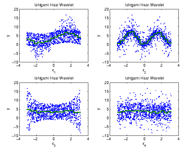
Example: Haar Wavelet on the Ishigami test data
|
Parameter | 1 | 2 | 3 | 4 |
|
0.3191 | 0.4138 | 0.0188 | 0.0148 |
These are exactly the same results as for CR. So was all of this brain strain for nothing? No,
using the Haar wavelet we can refine the
partition by including further wavelet coefficients.
The regression curves are still step functions: Do we find a better
orthogonal transformation?
Yes: The discrete cosine transformation (DCT) which is used for image compression in JPEG uses
continuous base functions.
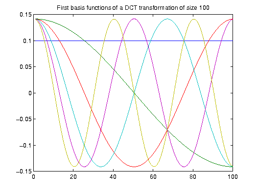
For example, the coefficient associated with the first base function, namely half a cosine wave
(green line),
almost provides the same information as a linear regression.
Example DCT
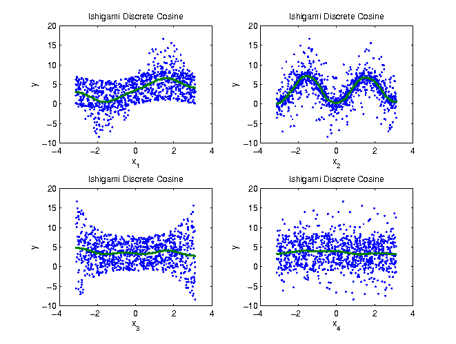
|
Parameter | 1 | 2 | 3 | 4 |
|
0.3121 | 0.4333 | 0.0162 | 0.0079 |
The DCT is a special case of the DFT with certain symmetry properties.
We can also directly apply the Fourier transformation by
sorting and shuffling the input values (Plischke, 2010):
By rearranging the order of realisations in the sample a
triangular shape can be constructed. Again, using this sorting procedure
an artificial timeframe is imposed on the sample. This method is termed EASI.
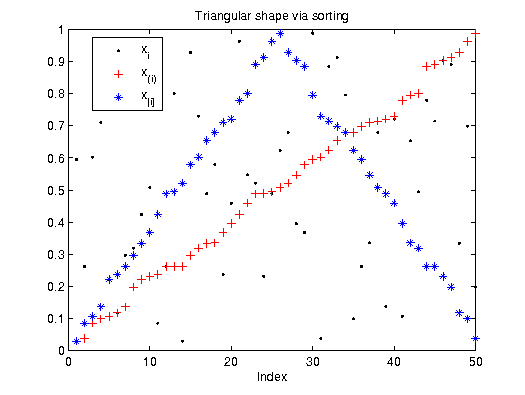
The rearranged input will show a triangular peak ("Mount Toblerone") so that resonances in
the accordingly rearranged output can be detected like in FAST and then attributed to the input factor.
Example EASI
We obtain
two regression curves, one from even indices and one from odd indices which gives us a visual feedback
on the quality of the fit and/or the data
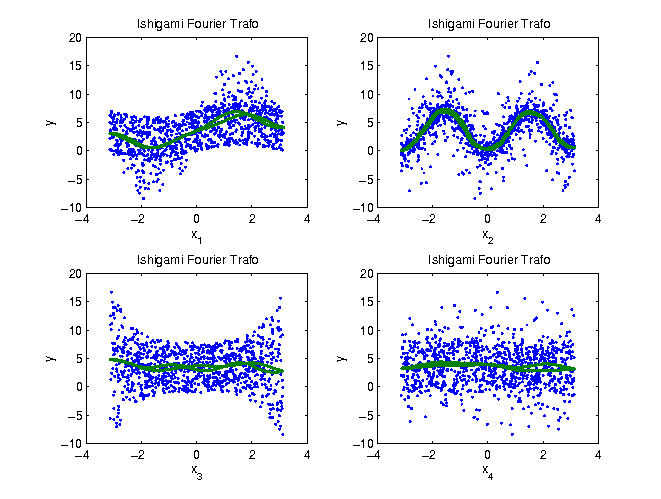
|
Parameter | 1 | 2 | 3 | 4 |
|
0.3172 | 0.4371 | 0.0218 | 0.0149 |
Second order effects (and higher if you dare)
Given data triplets
(as realisations of some RVs), we want to
compute the joint influence of
and on
The Method in a nutshell
- Sort the
input data along a search curve with a distinct frequency behaviour.
- Reorder output accordingly.
- Look out for resonances.
Plow Track Search Curve:
Code the
position by the length of the search curve going back and forth through
a checkerboard partition of the data.
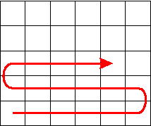
This curve has a detectable frequency behaviour per dimension, it can
easily extended to higher dimensions.
Ping-Pong Search Curve:
This is an alternative search curve design with large freedom of choosing the frequencies. Checkerboard sides have to be
incommensurable to reach all boxes.
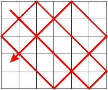
The quality of this length-assignment can be improved when using information on the exact position of the
realisation within the box.
Examples of search curve approaches
Rearranging the given realisations "like pearls on a string"
lets us perform a FAST analysis. Note that in contrast to the above analysis,
only a subset of the parameters is considered and the assignment to different frequencies is not fixed.
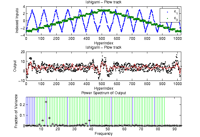
|
Parameter | 1 | 3 | 1,3 |
|
0.2864 | 0.0163 | 0.3154 |
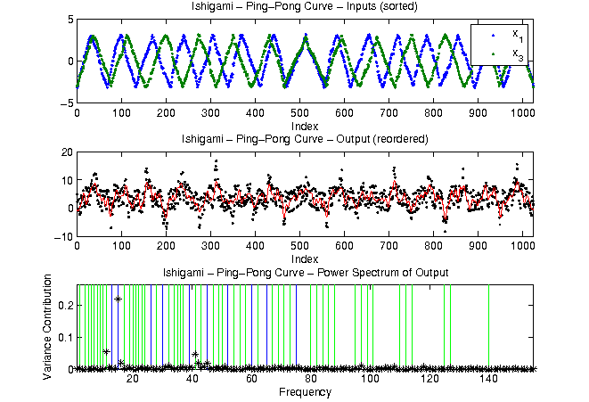
|
Parameter | 1 | 3 | 1,3 |
|
0.2424 | 0.0161 | 0.2327 |
Collecting the example results
The number of digits reported in the following table is a total overkill,
as the Monte Carlo error is approx.
| | 1 | 2 | 3 | 4 | 1,3 |
| | 0.19 | 0 | 0 | 0 | |
| Linear regression | 0.1936 | 0.0000 | 0.0026 | 0.0026 | |
| | 0.3139 | 0.4424 | 0 | 0 | 0.2437 |
| Correlation ratios | 0.3191 | 0.4138 | 0.0188 | 0.0148 | |
| Moving average | 0.3499 | 0.4564 | 0.0616 | 0.0420 | |
| HDMR | 0.3107 | 0.4500 | 0.0280 | 0.0070 | 0.2442 |
| FAST | 0.3076 | 0.4428 | 0.0000 | 0.0000 | 0.2435 |
| Haar wavelet | 0.3191 | 0.4138 | 0.0188 | 0.0148 | |
| DCT | 0.3121 | 0.4333 | 0.0162 | 0.0079 | |
| Fourier | 0.3172 | 0.4371 | 0.0218 | 0.0149 | |
| Plow-track | 0.2864 | | 0.0163 | | 0.3154 |
| Ping-pong | 0.2424 | | 0.0161 | | 0.2327 |
Note that the FAST method in this table uses a specially designed sample,
while the others always consider the same sample.
Open problems
The presented methods are computationally effective, but some questions remain open:
- Optimal Partition, Optimal number of coefficients
- Biased estimators
- Error bounds
- Best sample design for a method
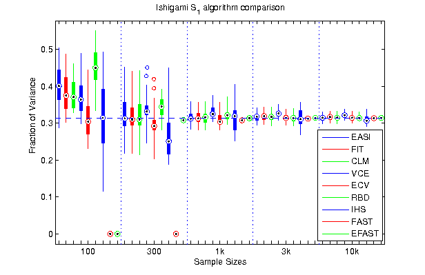
Estimating first order effects for first factor of Ishigami, 25 runs per sample size.
Density-based Sensitivity Measures
The variance of the conditional expectation is not a good indicator for multi-modal or highly skewed
conditional probability distributions.
Instead of comparing local means with the global mean, a moment-independent measure
should compare conditional densities with the unconditional one.
(Borgonovo, 2007) proposed to use the mean distance between the
conditional densities and the unconditional density
The -importance measure is symmetric in
and .
It is a -distance
of the product of the marginal pdfs and the joint pdf.
An estimator for
An efficient way of computing was until now out of reach.
Comparison with variance based sensitivity measure shows that
instead of the conditional mean
the conditional density
is needed for the estimation of density-based methods.
This requires to switch from pointwise distances to functional distances
where these functions have to be estimated from the given data.
We apply the same idea as for correlation ratios:
Replace the pointwise conditional density by a partition based
,
for suitable classes ,
by using kernel density estimates from the class data
Example: Ishigami function, parameter 2
Needs for the computation of
- Partition into classes
- Kernel density estimators
- Distance between densities
- Reduction of numerical errors using statistical tests
We discuss the highlighted items in the following.
Kernel density estimators
With a given kernel we define
The parameters ,
are called bandwidths or smoothing parameters
Suitable Kernels with mean 0 and variance 1
are:
|
Normal |
|
|
Triangle |
|
|
Epanechnikov |
|
|
Biweight |
|
|
Uniform |
|
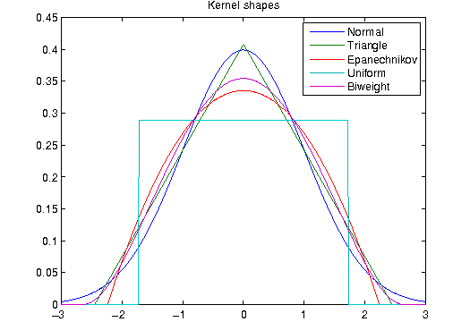
However, when performing numerical experiments one notices that it is not the shape which is important,
but the bandwidth selection for which there is a vast body of literature.
Kernel bandwidth
Results on optimal bandwidths are mostly available under the assumption of a Gaussian distribution.
For this, it is advantageous that
is invariant under monotonic transformations. Hence we can reshape the unconditional pdf to be Gaussian
by first passing from the original output data to the empirical cdf and then applying the inverse normal
cdf to the empirical cdf of the data. The optimal bandwidth derived for the unconditional pdf is then
also applied to compute the kernel density of the conditionals.
Difference of two densities
A theorem of [Scheffé 1947] shows that for all densities and
, we have
.
Choosing
shows that there is as much positive mass as there is negative mass in
.
This theorem links the measure to the
Kolmogorov-Smirnov distance ( restricted to half-rays)
and the discrepancy measure ( restricted to balls).
For kernel density estimates,
if
and
are close to each other then we expect many zeros crossings.
Hence it is difficult to apply advanced quadrature to the class separation
Hence we use the trapezoidal quadrature rule for numerical integration.
When are the densities the same?
The asymptotic Two-Sample Kolmogorov-Smirnov Test helps us in deciding whether
two densities are sufficiently
close to each other to yield a zero contribution:
If
and
denote the empirical cumulative distributions then
the contribution to is insignificant if
where is the (upper)
-quantile of the Kolmogorov distribution.
Typical values for are
,
,
,
especially,
for all .
The test is good in eliminating numerical dirt.
Moreover, the test statistics can be replaced with
using the above-mentioned theorem.
Ishigami Example, 8192 Quasi-MC samples
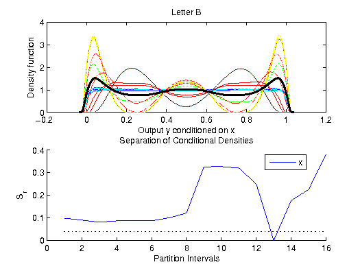
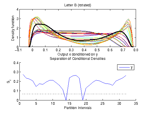
The following plots show the unconditional density of the output (fat) compared
to the densities conditioned on the inputs
(low x values: blue, high x values: red). The bottom plot shows the
separation between them.
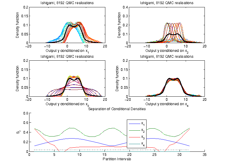
Generally, conditioning alters the density. Conditioning on factor 1
gives a shift in the density, factor 2 alters the shape completely,
factor 3 does not lead to a change in the conditional mean, but only
to the variance - a fact not detectable by variance-based first order
sensitivity indices. Factor 4 as a dummy only changes the shape
slightly. This slight changes are effectively eliminated by the
Kolmogorov-Smirnov test (Its cutoff value is marked with dots in the
lower plot). However, also some parts of factor 3 are effected by this cut-off.
|
Parameter | 1 | 2 | 3 | 4 |
| |
0.2037 | 0.3918 | 0.1392 | 0 |
|
| 0.3132 | 0.4365 | 0.0000
| 0.0000 |
Example: Letter B
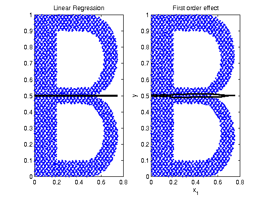
The data for the letter B was obtained by a rejection method. There are
no linear and no functional dependencies in the data, however, the plot definitely shows a structure.
Ideas, Problems, Open Issues
- Exchange the roles of and
- Non-equipopolated partitions (advanced quadrature for the outer loop)
- Use density of when available
- Kernel estimates for conditional densities with "all but the class
"
- Investigate on optimal bandwidth selection
- Use of Scheffé's Theorem for the separation between densities, e.g.,
consider zero crossings or only positive part
- Kolmogorov-Smirnov test to eliminate numerical dirt (test if densities are the same and
hence
)
- Higher order importance via search curves
- Bias? Consistency?
- Graphical methods for sensitivity
Conclusions
Computationally effective methods for the estimation of global sensitivity indicators
- are relatively easy to implement,
- offer advanced information compared to linear regression,
- based upon density estimates can use the same ideas as for variance-based estimators,
- are powerful when fed with Quasi Monte-Carlo sampling data.
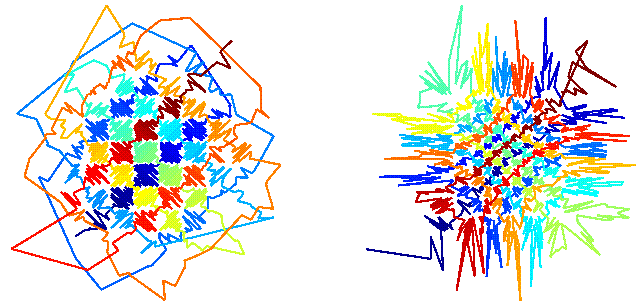
Search curves in action
References
(Saltelli et al., 2006) Sensitivity Analysis. Wiley&Sons, Chichester
(Pearson, 1905) On the General Theory of Skew Correlation and the Non-Linear Regression. Dulau&Co, London
(Pearson, 1912) On the General Theory of the Influence of Selection on
Correlation and Variation. Biometrika 8, 437-443
(Kolmogorov, 1933) Grundbegriffe der Wahrscheinlichkeitsrechnung. Springer, Berlin
(Plischke, 2010) An effective algorithm for computing global sensitivity indices (EASI).
Reliability Engineering&System Safety 95, 354-360
(Cukier et al., 1973) Study of the sensitivity of coupled reaction systems to
uncertainties in rate coefficients. J. Chem. Phys. 59, 3873-3878 3879-3888
(Borgonovo, 2007) A new uncertainty importance measure.
Reliability Engineering&System Safety 92, 771-784
(Rabitz&Alis, 1999) General foundations of high-dimensional model representations. J. Math. Chem. 25, 197-233
(Doksum&Samarov, 1995) Nonparametric estimation of global functionals and
a measure of the explanatory power of covariates in regression. The Annals of Statistics 23, 1443-1473